Session Seven: Sampling
This episode is a live recording of the seventh session of #UnblindingResearch held in DREEAM 19th September 2018. The group work has been removed for the sake of brevity.
This session of #UnblindingResearch looks at the factors that decide the sample size of our study. Here are the slides for this session (p cubed of course), you can move between slides by clicking on the side of the picture or using the arrow keys.


Here is the #TakeVisually for this session:
A population is the whole set of people in a certain area (say Britons). It is impossible to study a whole population so we have to use sampling. The 'target population' is the subset of the population we are interested in (such as Britons with hypertension). The sample is a further subset of the target population that we use as representative of the whole.
Generally every member of the population you are interested in should have an equal chance of being in the sample. Once an individual is included in the sample their presence shouldn't influence whether or not another individual is included.
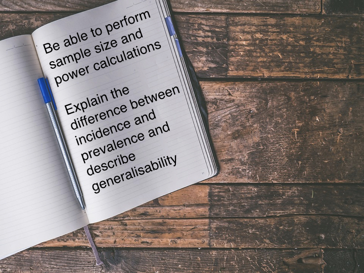
If our sample is too small we risk the study not being generalisable. If the sample is too big we risk wasting time, resources and exposing more participants to potential harm. So we have to get the right size through calculation.
For this session we looked at one population - Gummi Bears.

Just as with a human population Gummi Bears show variation across individuals. This could influence any study involving Gummi Bears. For the sake of this sessions we used a made up condition 'Red Gummi Fever' - a condition which makes Gummi Bears go red. We then thought about studying a potential cure. At the beginning we'd create a null hypothesis - that our new treatment would not cure Red Gummi Fever. As we make our null hypothesis we have to mindful of Type I error and Type II error
Type I error (false positive) - we falsely reject the null hypothesis (i.e. we say our cure works when it doesn't)
Type II error (false negative) - we falsely accept our null hypothesis (i.e. we say our cure doesn't work when it does)
Generalisability (or external validity) is the extent to which the findings of a study could be used in other settings. Internal validity is the extent to which a study accurately shows the state of play in the setting where it was held.

We also have to think about the condition itself and in particular its incidence and prevalence.
Incidence is the probability of occurrence of a particular condition in a population within a specified period of time. It is calculated by:
(Number of new cases in a particular period of time/Number of the population at risk of the event) - often expressed as number of events per 1000 or 10000 population
Prevalence is the number of cases of that disease in a particular population in a given time. It is calculated by:
(Number of cases in a population/total number of individuals in the population) - often expressed as a percentage but may be per 1000 or 10000 population for rarer conditions
So if we say we have a population of 1000 Gummi bears. 300 of them are red currently. Each year 50 bears catch red bear fever.
Our incidence is 50 events per 1000 population.
Our prevalence is 3%.

Back to our Type I and Type II Errors. When working out our sample size it is important that we have just the right amount of participants to overcome these errors.
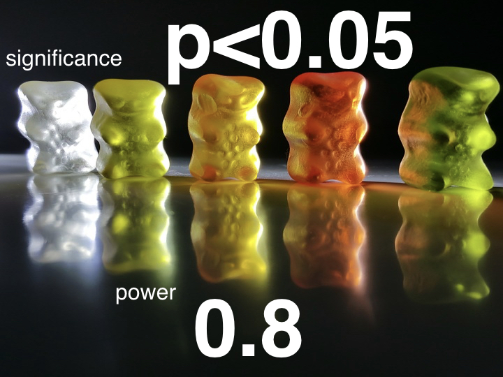
Significance is concerned with Type I Error. We ask ourselves the question "could the effect I've seen have occurred at random?" It is expressed with a p value. A p value of 0.05 means that there is a 5% chance of the study outcome have occurring at random. The gold standard is a p value <0.05. So when we are working out our sample size for our treatment for red bear fever we want it to be able to have a p value <0.05 so if our study finds that our treatment works we can say there is a less than 5% chance that our finding was down to chance alone. A p value >0.05 is not deemed significant.
When thinking about significance a test can be one or two tailed. This is all to do about what we are hoping to show.
For example, you might have developed a new drug to treat hypertension. You would trial it against the current standard of hypertensive treatment. If you were only interested in a non-inferior outcome (i.e. you just want to show your new drug isn’t worse than the current gold standard) then you’d only need a one tailed test. Your p value would be totally allotted to that one outcome. If you wanted to show that your new drug is both better and not worse (a superior and non-inferior) outcome then you would need a two tail test. Half of your p value would be allotted to the non-inferior outcome and half to your superior outcome.
Power is concerned with Type II Error. Here we ask ourselves "what is the chance of us falsely finding a negative outcome?" This is expressed as a decimal. Power of 0.8 (or 80%) means there is a 20% chance (or 1/5) of a falsely negative result being found. 0.8 is the usual gold standard while some larger/pivotal studies will want a power of 0.9.

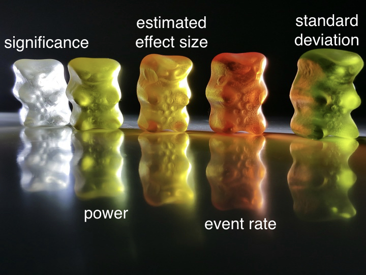
What we then have to consider are estimated effect size, the event rate and the standard deviation of our population.
Estimated effect size = Effect size this is essentially what we want our treatment to do. This is calculated by the control variable minus the test variable. This could be a reduction in mortality, in blood pressure etc. Estimated effect size is based on previously reported or pre-clinical studies. The larger the effect size in previous groups the smaller our sample needs to be. The smaller our effect size the larger the sample needs to be.
The underlying event rate or prevalence. We take this from previous studies.
We finally need to know how varied our population is. Standard deviation is a measure of the variability of the data. The more homogenous our population the smaller the variation and so the smaller the standard deviation means our sample size needs to be smaller.

The calculations to work out a sample size are quite complicated so luckily there is software and several websites we can use to help us. This link goes to one such example at ClinCalc which shows everything we've talked about here quite nicely.
Here are a couple of papers which go through sample sizes:
While we’re still thinking about power and significance it’s worth thinking about fragility index. Fragility Index looks at how many events would need to change for the p value to go >0.05 (how many events need to change for the outcome to no long be significant). The lower the Fragility Index the more fragile the study is. This is important because a lot of clinical trials actually turn out to be very fragile.
A Fragility Index calculator is available here
Say you’ve studied 100 people on new treatment vs 100 on the old treatment
Intervention mortality was 7 whilst control mortality was 20
Using the above calculator we find we’d only need 3 events to change for our trial to no longer be significant
More on fragility index here